Introduction
A recent blog article introduced me to the idea of double descent. This is the phenomenon by which the fitting error in the testing set of a (presumably gradient descent-based) machine-learning method goes down as the number of parameters increases, then rises again (a phenomenon known as overfitting), but then goes down again as the number of parameters is increased still further. I do not want to comment on the specifics of this article as they pertain to machine learning, but rather on a sub-aspect of it.
In short, the authors want to make the point that as long as the fitting error in the testing set decreases, it doesn’t matter whether the number of parameters is increased beyond any reasonable amount. I wish to respectfully disagree.
Fitting Polynomials (By Least Squares)
The Example Data Set
To illustrate the phenomenon of double descent, the authors use synthetic data that. (Thanks are due to the authors, who published their data in a notebook.) First, here is a plot of the data set in question, together with a linear model, i.e., a straight line that minimises (in a certain way) the difference between the data points and the line.

Example data set used in this example.
Fitting a Straight Line
This straight line, to no-one’s surprise, results in a rather bad fit. I say that this happens “to no one’s surprise” because the plot makes it clear that the ground truth is not a straight line.
However, first of all, in this instance the linear model may not be a good fit, but it’s not a terrible fit either. The linear model has a slope that seems to fit the data quite well, which becomes apparent when we look at the residuals:

Residuals when fitting a straight line.
This is also evidenced by a t-test on those residuals:
> summary(m)

Call:
lm(formula = y ~ x)

Residuals:
     Min       1Q   Median       3Q      Max
-0.96265 -0.31533 -0.03154  0.34024  0.86479

Coefficients:
            Estimate Std. Error t value Pr(>|t|)
(Intercept)  -0.0300     0.1146  -0.262 0.796403
x            -0.8348     0.1888  -4.423 0.000328 ***
---
Signif. codes:  0 ‘***’ 0.001 ‘**’ 0.01 ‘*’ 0.05 ‘.’ 0.1 ‘ ’ 1

Residual standard error: 0.5124 on 18 degrees of freedom
Multiple R-squared:  0.5208,	Adjusted R-squared:  0.4942
F-statistic: 19.56 on 1 and 18 DF,  p-value: 0.0003285
Now obviously, the fit of the slope isn’t perfect; it can’t be. But the question is, is that because the data has random noise in it or because the model is wrong? In order to shed light on this question, we look at a Q-Q plot of the residuals.
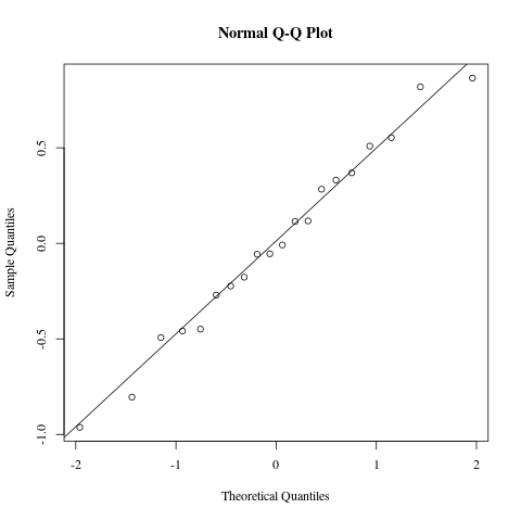
Q-Q plot of residuals of linear model.
This plot shows that the residuals are very nicely normally distributed, so case closed, right? The data is essentially linear, with a random perturbation. Bot not so fast! The residuals plot dispels the notion that the residuals are random. There is an obvious functional relationship between $x$ and the residual at $x$, and the residuals are large. This shows conclusively that the linear model is not right, even though the Q-Q plot and the t-test on the residuals say that the fit is good.
How come this fits so well if the model is wrong? Stand by, that’s going to be the subject of the next paragraph. But at any rate, we can already learn something about our data: over about half of its range, from about $-0.5$ to $0.5$, it is very nearly linear, with slope $-1$ (analysis not shown).
Fitting a Third-Degree Polynomial
But look again at the graph of the data. Does this look like some ground truth where all points have been perturbed by random (i.e., normal) noise? No. What it looks like is some curve where some points are perturbed by non-normal noise. And looking at the code that generated the data, this is exactly what we see:
n = 20
sigma = 0.3 # stdev of noise

def cubic_gt(x):
  return poly(x, np.array([0, -1, 0, 1]), 3)

ground_truth = cubic_gt

G = np.polynomial.legendre.legvander # Legendre polynomial basis

def poly(pts, beta, d):
  return G(pts, d).dot(beta)

## Compute ground-truth polynomial + noise

x = np.linspace(-1, 1, n)
y = ground_truth(x)

y += (rand.uniform(size=n) <= 0.2)*sigma # random L0 noise
y -= (rand.uniform(size=n) <= 0.1)*2*sigma # random L0 noise
So it turns out that the ground truth in this case is $y = x^3 - x$ in the range $-1$ to $1$. And this, over about half its range, from about $-0.5$ to $0.5$, is not a third-degree polynomial at all, it’s $y = -x$ with some third-degree perturbation that becomes increasingly irrelevant as $x \to 0$. This explains our observations above very well.
Also, it’s not that all points are perturbed by random noise, only some points are, and if they are perturbed, they are perturbed systematically by $+\sigma$ (with probability $0.2$) or $-2\sigma$ (with probability $0.1$). I am not an expert, so I don’t know how common this kind of noise is, but it is certainly not normal. But least squares is not designed to deal with non-normal noise, so the method does not fit the data! (I’m not referring to the mathematical method of least squares fitting, which after all does not care what its input looks like. I am referring instead to the use of it in statistics, where normally distributed errors are taken as a sign that you have found the correct model.)
Some people may say that I’m missing the point because this is just some stupid example data, quickly created to make another point later on. On the contrary, I think that this illustrates a rather cavalier attitude to data, which is ironic in something in a discipline that has the word “data” right there in its name. I believe with all my heart that details matter and that if you are about to unleash an algorithm on some data, it’s your duty to make sure that the algorithm is appropriate. If the algorithm is not appropriate, you get garbage out, simply because you put garbage in. It is often not appreciated that this principle not only applies when the data are garbage, but when the method is.
The second point I want to make is that I believe that the authors, together with many machine-learning enthusiasts, are rather, in my opinion, missing the point of machine learning. If we take “machine learning” at face value, the objective of machine learning is learning. What has the machine learned when it has found the line that creates the smallest quadratic residuals? Without appreciating the form of those residuals, arguably nothing.
Let’s now look at the residuals from cubic interpolation.
Residuals from cubic interpolation of the test data.
Q-Q plot from cubic interpolation of the test data.


The residuals here also show a clear functional relationship; the residuals are again not random. In this case, they aren’t even normally distributed, as the Q-Q plot clearly shows. But in this case, the residuals are generally small, and they are large for only a few points. Coincidentally (not!), these points are also the points that spoil the otherwise good fit of the Q-Q plot. These are the points that are so far outside that they could be treated as outliers, provided that we have looked at the points and concluded that they are indeed outliers.
If we remove these points from the data set, we get a perfect fit. Of course, knowing how the data set was created, this is not surprising. (If you think that the nonzero residuals or the bad Q-Q plot mean that the fit is not perfect, think again.) We have again learned something about our data set: the data consists of a cubic polynomial, plus a few outliers.
Residuals from cubic interpolation of the test data, with outliers removed.
Q-Q plot from cubic interpolation of the test data, with outliers removed.

What We Have Learned With Polynomials of Degree At Most 3
To summarise, here is what we can learn from the data:
- The data is very nearly linear from $-0.5$ to $0.5$.
- In that realm, the data is very well approximated by a straight line with slope $-1$.
- The data contains a few outliers.
- Removing them gives a perfect fit with $y = x^3 - x$.
This means that the third-degree polynomial is the correct model for the data and trying to look for other models is futile, as long as there is no theory that suggests that other models should be tried or that the outliers are in fact not outliers.
This immediately suggests two ways to continue to analyse the data:
- For those points that are perfectly fitted with a third-degree polynomial, find a possible hypothesis that would explain this unusually precise relationship.
- For the outliers, look at whether they really belong to the data set from which the other data points are coming, or whether they might not be from another data set altogether. If they are indeed from the same data set, i.e., if $y = x^3 - x + \epsilon$, what could explain this non-normal noise $\epsilon$?
This, I suggest, is learning.
Fitting a Thousandth-Degree Polynomial
Now the authors of the paper go further. After having fitted a third-degree polynomial, and after having conceded that this is the “correct” (their words) fit, they try higher and higher degrees to illustrate overfitting, which means that the residuals for the training set goes down, but the residuals for the testing set goes up. In this case, this happens because if the testing set indeed comes from $y = x^3 - x$, then the higher the degree of polynomial you force to go through certain points, the more that polynomial will deviate from the correct one. When the $x$ values are equidistant, as is the case here, this will happen especially at the boundary of the region to be fitted. It should be noted that after degree $3$, the fitting error for the training set will be exactly zero. This is not rocket science, being instead among the topics of any undergraduate course on numerical analysis.
The authors are however undeterred and fit higher and higher polynomials until they finally arrive at a 1000-degree polynomial. There they see that the fitting errors for a testing set will go down again. This is known as double descent: the fitting error goes down as you approach the correct (or at any rate best) model, goes up as you get away from it, but then goes down again as you in increase the number of parameters to be fitted beyond any reasonable amount.
The authors now say that this phenomenon means that overfitting by using massively more parameters than necessary isn’t bad, as long as it makes the residuals smaller:
We still fit all the training points, but now we do so in a more controlled way which actually tracks quite closely the ground truth. We see that despite what we learn in statistics textbooks, sometimes overfitting is not that bad, as long as you go ‘all in’ rather than “barely overfitting” the data. That is, overfitting doesn’t hurt us if we take the number of parameters to be much larger than what is needed to just fit the training set — and in fact, as we see in deep learning, larger models are often better.
Well yes, they will fit all training points, but if the training points contain error (a standard assumption when fitting models, and indeed the method for generating the data in this very example), this is exactly what you do not want. You will fit the error, and that’s not any good to anyone. Also note that the assertion that “ground truth is closely tracked” is true, but it’s even more true for the third-degree polynomial than the 1000-degree polynomial, would be even better for a piecewise linear function, and is perfect for the third-degree polynomial with outliers removed.
As I will elaborate below, there are two more reasons why this attitude is just wrong, one mathematical and one philosophical.
First, fitting a 1001-parameter model is the perfect excuse (if an excuse is actually needed) to quote Forman S. Acton. Acton emphasised deep and detailed knowledge of data and behaviour of functions over blind application of methods. In his 1970 book Numerical Methods That (usually) Work, he writes:
[Researchers that try to fit a 300-parameter model by least squares] leap from the known to the unknown with a terrifying innocence and the perennial self-confidence that every parameter is totally justified. It does no good to point out that several parameters are nearly certain to be competing to “explain” the same variations in the data and hence the equation system will be nearly indeterminate. It does no good to point out that all large least-squares matrices are striving mightily to be proper subsets of the Hilbert matrix—which is virtually indeterminate and uninvertible—and so even if all 300 parameters were beautifully independent, the fitting equations would still be violently unstable.
What does this mean? It means that the concrete values of those 1001 coefficients are meaningless because there are tons of other values that give a similar small residual error when used for prediction.
Now you may argue that this is irrelevant because in machine learning, we do not believe that “every parameter is totally justified”. That’s because all you are interested in is the size of the residuals, not the concrete parameter values. But the residuals are smallest when you fit a third-degree polynomial and remove outliers!
If this is not enough for you, there is another reason. Acton continues in Numerical Methods that (usually) Work:
Most of this instability is unnecessary, for there is usually a reasonable procedure. Unfortunately, it is undramatic, laborious, and requires thought […]. They should merely fit a five-parameter model, then a six-parameter one. If all goes well and there is a statistically valid reduction of the residual variability, then a somewhat more elaborate model may be tried. Somewhere along the line—and it will be much closer to 15 parameters than to 300—the significant improvement will cease and the fitting operation is over. […] The computer center’s director must prevent the looting of valuable computer time by these would-be fitters of many parameters.
And here is the true crux of the matter. The fact is that you cannot learn anything from a 1001-parameter model that you couldn’t also learn from a 3- (or 4- or 5- or even 15-) parameter model. If the objective is to reduce the residual error when fitting the testing set, you’re better off with a third-degree polynomial (or even a piecewise linear function for heaven’s sake). If the objective is to find meaning in any of the parameters, i.e., to assign them to some influence in the real world, then you are also better off with a four-parameter model than with a 1001-parameter one.
STOP OVERFITTING YOUR DATA, IT MAKES NO SENSE!
(Source code for the graphs and analyses in this post available here.)